This page was generated from rem.ipynb. Interactive online version:

Relative Elevation Model

This tutorial is inspired by this blog post, this excellent story map, and this notebook.

from pathlib import Path

import matplotlib.pyplot as plt
import numpy as np
import shapely.ops as ops
import xarray as xr
import xrspatial as xs
from datashader import transfer_functions as tf
from datashader import utils as ds_utils
from datashader.colors import Greys9, inferno
from scipy.spatial import KDTree

import py3dep
import pynhd

import warnings

warnings.filterwarnings("ignore", ".*invalid value encountered in.*")

Relative Elevation Model (REM) detrends a DEM based on the water surface of a stream. It’s especially useful for visualization of floodplains. We’re going to compute REM for a segment of Carson River and visualize the results using xarray-spatial and datashader.

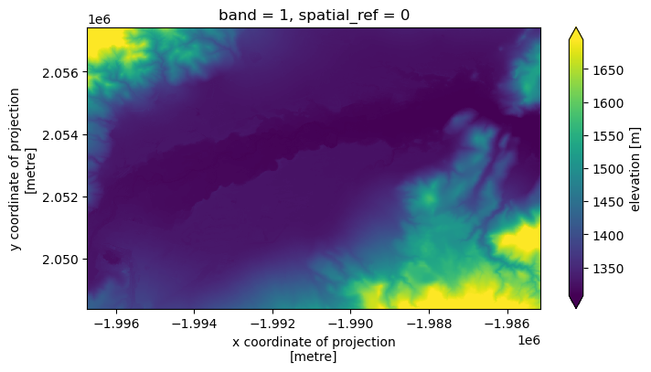
First, let’s check out the available DEM resolutions in our area of interest (AOI).

bbox = (-119.59, 39.24, -119.47, 39.30)
dem_res = py3dep.check_3dep_availability(bbox)
dem_res

{'1m': True,
 '3m': False,
 '5m': False,
 '10m': True,
 '30m': True,
 '60m': False,
 'topobathy': False}

We can see that Lidar (1-m), 10-m, and 30-m are available. Obviously, Lidar data gives us the best results, but it can be computational expensive. So, we’re going to set the resolution 5 m since 1-m and 10-m data are available.

res = 5
dem = py3dep.get_map("DEM", bbox, res)

fig, ax = plt.subplots(figsize=(8, 4), dpi=100)
_ = dem.plot(ax=ax, robust=True)

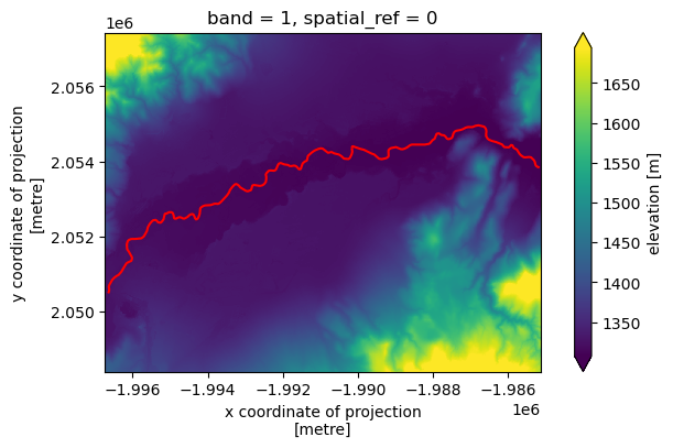
Next, we need to get the river’s centerline. For this purpose, first we get the flowlines within our AOI. Then, we remove all the isolated flowlines using the remove_isolated flag of pynhd.prepare_nhdplus and find the main flowline based on the minimum value of the levelpathi attribute.

wd = pynhd.WaterData("nhdflowline_network")

flw = wd.bybox(bbox)
flw = pynhd.prepare_nhdplus(flw, 0, 0, 0, remove_isolated=True)
flw = flw[flw.levelpathi == flw.levelpathi.min()].copy()

fig, ax = plt.subplots(figsize=(8, 4), dpi=100)
flw.plot(ax=ax, color="r")
_ = dem.plot(ax=ax, robust=True)

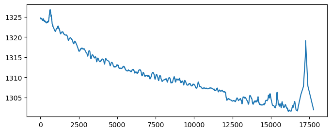
Now, we can get the elevation profile along the obtained main flowline with spacing of 10 meters.

lines = ops.linemerge(flw.geometry.tolist())
riv_dem = py3dep.elevation_profile(lines, 10, crs=flw.crs)
_ = riv_dem.plot(x="distance", figsize=(7, 3.2))

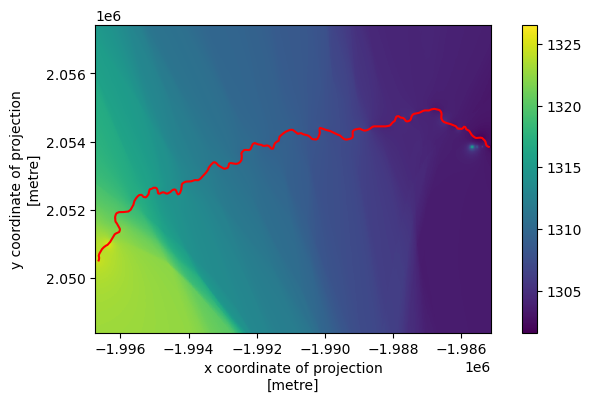
There are several methods for detrending the DEM based on the river’s elevation profile. You can check these method in this poster. Here, we’re going to use Inverse Distance Weighting method using scipy’s KDTree function and setting the number of neighbors to 200.

def idw(riv_dem: xr.DataArray, dem: xr.DataArray, n_nb: int) -> xr.DataArray:
    """Interpolate grid DEM from river DEM using Inverse Distance Weighting."""
    riv_coords = np.column_stack((riv_dem.x, riv_dem.y))
    kdt = KDTree(riv_coords)

    dem_grid = np.dstack(np.meshgrid(dem.x, dem.y)).reshape(-1, 2)
    distances, idx = kdt.query(dem_grid, k=n_nb)

    weights = np.reciprocal(distances)
    weights = weights / weights.sum(axis=1, keepdims=True)

    interp = weights * riv_dem.to_numpy()[idx]
    interp = interp.sum(axis=1).reshape((dem.sizes["y"], dem.sizes["x"]))
    return xr.DataArray(interp, dims=("y", "x"), coords={"x": dem.x, "y": dem.y})


elevation = idw(riv_dem, dem, 200)
rem = dem - elevation

fig, ax = plt.subplots(figsize=(8, 4), dpi=100)
elevation.plot(ax=ax)
_ = flw.plot(ax=ax, color="red")

Let’s use datashader to stack DEM, Hillshade and REM for a nice visualization. There are a couple of parameters in this tutorial that can be change for extending it to other regions: Number of neighbors in IDW, DEM resolution, span argument of REM’s shading operation.

illuminated = xs.hillshade(dem, angle_altitude=10, azimuth=90)
tf.Image.border = 0
img = tf.stack(
    tf.shade(dem, cmap=Greys9, how="linear"),
    tf.shade(illuminated, cmap=["black", "white"], how="linear", alpha=180),
    tf.shade(rem, cmap=inferno[::-1], span=[0, 7], how="log", alpha=200),
)
ds_utils.export_image(img[::-1], Path("_static", "rem").as_posix())