This page was generated from flood_peak.ipynb.
Interactive online version:
![]()
Flood Moments for CAMELS#
In this tutorial, we learn about computing three statistical flood moments, namely, mean annual flood (MAF), coefficient of variation (CV), and skewness (CS) for all 671 USGS gage stations that are included in the CAMELS dataset.
[1]:
from __future__ import annotations

from pathlib import Path

import cytoolz as tlz
import matplotlib.pyplot as plt
import numpy as np
import pandas as pd

import pygeohydro as gh
First, we use pygeohydro.get_camels to get the CAMELS dataset. This function returns one geopandas.GeoDataFrame containing basin geometries of the stations and 59 other basin properties, and a xarray.Dataset containing streamflow values and the same 59 basin properties. Essentially, the difference between the two is that one has basin geometries and the other has streamflows.
[2]:
camels_basins, camels_qobs = gh.get_camels()
Now, let’s extract the station IDs, their drainage area, and start and end dates of the streamflows.
[3]:
area_sqkm = camels_qobs.area_geospa_fabric.to_series()
start = camels_qobs.time[0].dt.strftime("%Y-%m-%d").item()
end = camels_qobs.time[-1].dt.strftime("%Y-%m-%d").item()
station_ids = camels_basins.index
Next, instead of using mean daily streamflow data from the CAMELS dataset, we use NWIS’s peak streamflow service. The pygeohydro.NWIS class has a method called retrieve_rdb for pulling data from NWIS services in the RDB format. This function is very handy for sending requests to NWIS and processing the responses to a pandas.DataFrame.
The peak streamflow service accepts multiple station IDs per request by using multiple_site_no keyword. However, since the service uses the GET request method, there’s a limit on the number of characters per request. Thus, we need to partition our station IDs into smaller chunks per request. We use cytoolz library for this purpose.
[4]:
nwis = gh.NWIS()

base_url = "https://nwis.waterdata.usgs.gov/nwis/peak"
payloads = [
    {
        "multiple_site_no": ",".join(sid),
        "search_site_no_match_type": "exact",
        "group_key": "NONE",
        "sitefile_output_format": "html_table",
        "column_name": "station_nm",
        "begin_date": start,
        "end_date": end,
        "date_format": "YYYY-MM-DD",
        "rdb_compression": "file",
        "hn2_compression": "file",
        "list_of_search_criteria": "multiple_site_no",
    }
    for sid in tlz.partition_all(100, station_ids)
]
peak = nwis.retrieve_rdb(base_url, payloads)[["site_no", "peak_dt", "peak_va"]]
Next, we extract year from the peak_dt column and covert peak_va to float. Also, peak_va is in cubic feet per second and for computing the flood moments we need to convert it into cubic meter per second per square km using the stations’ upstream drainage area.
[5]:
peak["year"] = peak.peak_dt.str.split("-").str[0].astype(int)
peak["peak_va"] = pd.to_numeric(peak.peak_va, errors="coerce")
peak = peak.groupby(["year", "site_no"]).peak_va.max()
peak = peak.unstack(level=1) * 0.3048**3 / area_sqkm
Since there are missing values in our data let’s use CAMEL’s dataset to fill those.
[6]:
print(
    "No. of missing values in data from Peak Streamflow service: ",
    peak.isna().sum().sum(),
)
No. of missing values in data from Peak Streamflow service: 3440
[7]:
camels_peak = camels_qobs.discharge.to_series()
camels_peak = (
    camels_peak.reset_index().set_index("time").groupby(["station_id", pd.Grouper(freq="Y")]).max()
)
camels_peak = camels_peak.unstack(level=0)
camels_peak.index = camels_peak.index.year
camels_peak.columns = camels_peak.columns.droplevel(0)
camels_peak = camels_peak * 0.3048**3 / area_sqkm
[8]:
print(
    "No. of missing values in data from CAMELS dataset: ",
    camels_peak.isna().sum().sum(),
)
No. of missing values in data from CAMELS dataset: 463
[9]:
peak = peak.fillna(camels_peak)
[10]:
print(
    "No. of missing values after the filling operation: ",
    peak.isna().sum().sum(),
)
No. of missing values after the filling operation: 392
The peak streamflow data is now ready to be used for computing the flood moments.
[11]:
def compute_flood_moments(annual_peak: pd.DataFrame) -> pd.DataFrame:
    """Compute flood moments (MAF, CV, CS) from annual peak discharge values."""
    maf = annual_peak.mean()
    n = annual_peak.shape[0]
    s2 = np.power(annual_peak - maf, 2).sum() / (n - 1)
    cv = np.sqrt(s2) / maf
    cs = n * np.power(annual_peak - maf, 3).sum() / ((n - 1) * (n - 2) * np.power(s2, 3.0 / 2.0))

    fm = pd.concat([maf, cv, cs], axis=1)
    fm.columns = ["MAF", "CV", "CS"]
    return fm


fm = compute_flood_moments(peak)
Lastly, let’s merge the obtained flood moments with the basin geometries for visualization.
[12]:
basins = camels_basins.to_crs(5070).geometry.centroid.to_frame("geometry")
camels_fm = basins.merge(fm, left_index=True, right_index=True)
We can use the pygeohydro.helpers.get_us_states to get the CONUS states geometries.
[13]:
conus = gh.helpers.get_us_states("contiguous").to_crs(camels_fm.crs)
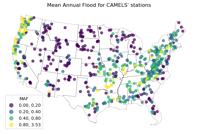
[14]:
fig, ax = plt.subplots(figsize=(8, 8), dpi=100)
ax.set_title("Mean Annual Flood for CAMELS' stations")
conus.plot(ax=ax, facecolor="none", edgecolor="black", linewidth=0.2)
camels_fm.plot(
    ax=ax,
    column="MAF",
    scheme="User_Defined",
    legend=True,
    cmap="viridis",
    alpha=0.7,
    classification_kwds={"bins": [0.2, 0.4, 0.8]},
    legend_kwds={"title": "MAF", "ncols": 1},
)
ax.set_axis_off()
fig.savefig(Path("_static", "flood_peak.png"), dpi=300)
We can also use explore function of geopandas to plot an interactive map of the results.
[15]:
def plot_flood_moments(column):
    """Plot flood moments (MAF, CV, CS) from annual peak discharge values."""
    vmin, vmax = camels_fm[column].quantile([0.1, 0.9])
    return camels_fm.explore(
        column=column,
        vmin=vmin,
        vmax=vmax,
        cmap="viridis",
        marker_kwds={"radius": 4},
        style_kwds={"stroke": False},
    )
[16]:
plot_flood_moments("CV")
[16]:
[17]:
plot_flood_moments("CS")
[17]: