This page was generated from hymod_calibration.ipynb. Interactive online version:

Making Waves in Water Science: Open Source Tools

Hosted by CUAHSI

HyRiver: Hydroclimate Data Retriever

Presenter: Taher Chegini, University of Houston

Email: cheginit@gmail.com

Nov 6th, 2022

Introduction

The traditional approach for retrieving hydroclimate data from different source was mostly as follows:

• Download entire datasets from various data sources to a local workstation

• Process the data and subset for the region of interest on the workstation

• Store the processed input data and the analyses results locally

• Upload the data to a remote server for publication and sharing

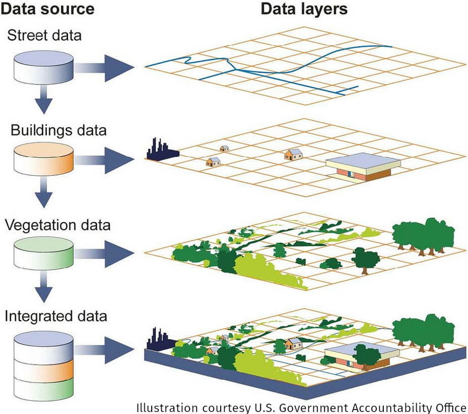
Over the last decade using web services have become more common in the geospatial community.

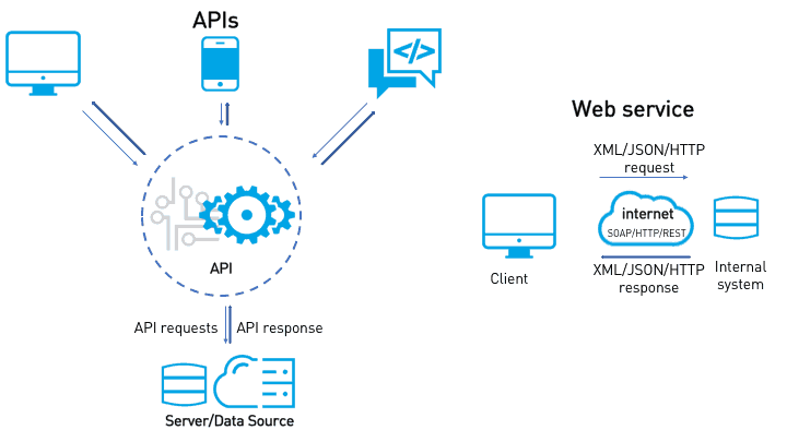
Image source

HyRiver is a suite of eight open-source (MIT License) Python packages that bridges the gap between (non-technical) hydrologists and complexities of working with web services. Contribution of any kind are most welcome.

Package	Description
	Navigate and subset NHDPlus (MR and HR) using web services
	Access topographic data through National Map’s 3DEP web service
	Access gNATSGO, NWIS, NID, WQP, HCDN 2009, NLCD, CAMELS, and SSEBop databases
	Access daily, monthly, and annual climate data via Daymet
	Access hourly NLDAS2 forcing data
	A collection of tools for computing hydrological signatures
	High-level API for asynchronous requests with persistent caching
	Send queries to any ArcGIS RESTful-, WMS-, and WFS-based services
	Utilities for manipulating geospatial, (Geo)JSON, and (Geo)TIFF data

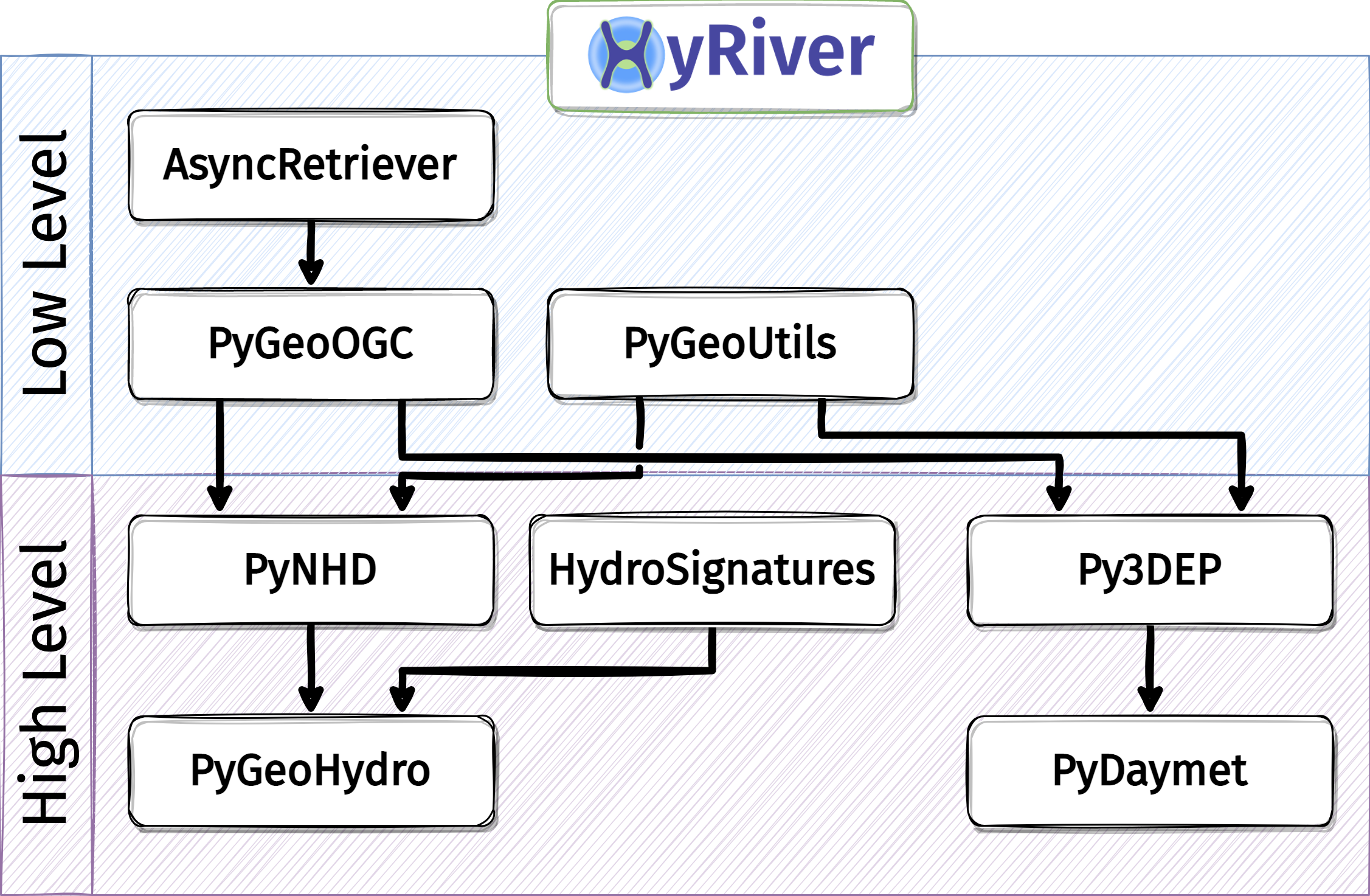
Here’s a chart of HyRiver packages dependencies:

An Application in Hydrological Modeling

from pathlib import Path

import contextily as ctx
import numpy as np
import pandas as pd
from hymod import HYMOD
from scipy import optimize

import pydaymet as daymet
import pygeohydro as gh
import pygeoutils as geoutils
from pygeohydro import NWIS
from pynhd import NLDI

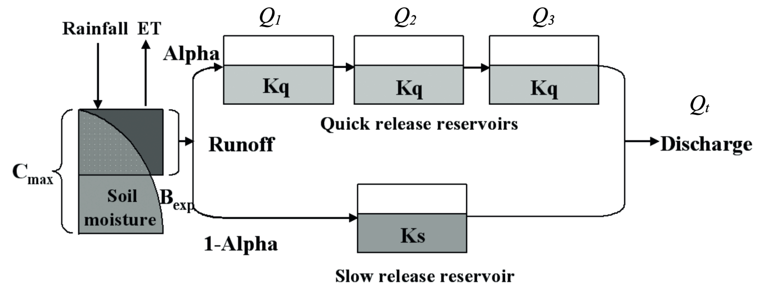
We use HyRiver packages to get the required input data for hydrological modeling of a watershed. We use PyDaymet to get precipitation and potential evapotranspiration and PyGeoHydro to get streamflow observations and soil storage capcity. Then, we use an implementation of the HYMOD model for our watershed analysis. The source for the model can be found in hymod.py file.

First, we use the CAMELS dataset to select a natural watershed with no significant snow since this implementation of HYMOD does not have a snow component.

camels_basins, camels_qobs = gh.get_camels()

stations = camels_basins[
    (camels_basins.area_gages2 > 300)
    & (camels_basins.area_gages2 < 500)
    & (camels_basins.frac_snow < 0.1)
]
station = stations.iloc[0].name

Next, we get more information about our selected watershed drainage area geometry using PyNHD and PyGeoHydro. To ensure that the station is located at the outlet of the watershed, we set split_catchment flag to True to split the catchment at the station’s location.

dates = ("2003-01-01", "2012-12-31")
nwis = NWIS()

basin = NLDI().get_basins(station, split_catchment=True)
info = nwis.get_info({"site": station})
info

	agency_cd	site_no	station_nm	site_tp_cd	dec_lat_va	dec_long_va	coord_acy_cd	dec_coord_datum_cd	alt_va	alt_acy_va	alt_datum_cd	huc_cd	nhd_id	nhd_areasqkm	hcdn_2009	geometry
0	USGS	01666500	Robinson River Near Locust Dale, VA	ST	38.32513	-78.095556	U	NAD83	282.64	0.08	NAVD88	02080103	8468559	463.61	True	POINT (-78.09556 38.32513)

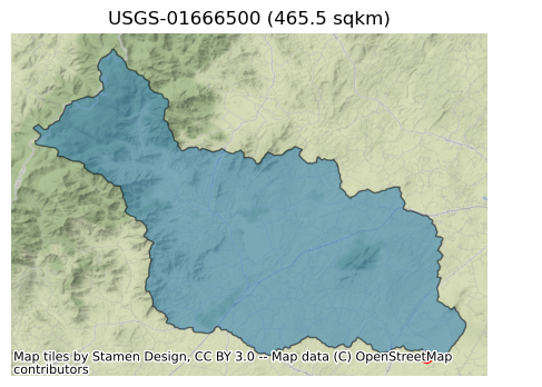
Let’s check the area of the watershed and plot it.

area_sqm = basin.to_crs(basin.estimate_utm_crs()).area.values[0]
ax = basin.plot(figsize=(9, 4), alpha=0.5, edgecolor="black")
info.plot(ax=ax, markersize=50, color="red")
ax.set_title(f"USGS-{station} ({area_sqm * 1e-6:.1f} sqkm)")
ctx.add_basemap(ax, crs=basin.crs)
ax.margins(0)
ax.set_axis_off()
ax.figure.savefig(Path("_static", "hymod.png"), dpi=300, bbox_inches="tight", facecolor="w")

Now, we get some information about this station and then retrieve streamflow observations within the period of our study for calibrating the model from PyGeoHydro. Since HYMOD’s output is in mm/day we can either set the mmd flag of NWIS.get_streamflow to True to return the data in mm/day instead of the default cms, or use area_sqm that we obtained previously to do the conversion. Note that these two methods might not return identical results since NWIS.get_streamflow uses GagesII and NWIS to get the drainage area while here we used NLDI to obtain the area and these two are not always the same.

qobs = nwis.get_streamflow(station, dates)
qobs = qobs * (1000.0 * 24.0 * 3600.0) / area_sqm

We can check the difference in areas produced by these two methods as follows:

area_nwis = nwis._drainage_area_sqm(info, "dv")
f"NWIS: {area_nwis.iloc[0] * 1e-6:.1f} sqkm, NLDI: {area_sqm * 1e-6:.1f} sqkm"

'NWIS: 463.6 sqkm, NLDI: 465.5 sqkm'

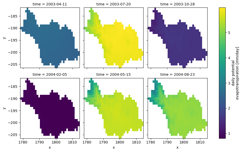
PyDaymet can compute Potential EvapoTranspiration (PET) at daily timescale using three methods: penman_monteith, priestley_taylor, and hargreaves_samani. Let’s use hargreaves_samani and get the data for our study period.

clm = daymet.get_bygeom(basin.geometry[0], dates, variables="prcp", pet="hargreaves_samani")

_ = (
    clm.where(clm.pet > 0)
    .pet.isel(time=range(100, 700, 100))
    .plot(x="x", y="y", row="time", col_wrap=3)
)

Since our HYMOD implementation is a lumped model, we need to take the areal average of the input precipitation and potential evapotranspiration data. Moreover, since Daymet’s calendar doesn’t have leap years (365-day year), we need to make sure that the time index of the input streamflow observation matches that of the climate data.

clm_df = clm.mean(dim=["x", "y"]).to_dataframe()[["prcp", "pet"]]
clm_df.index = pd.to_datetime(clm_df.index.date)

qobs.index = pd.to_datetime(qobs.index.to_series().dt.tz_localize(None).dt.date)
idx = qobs.index.intersection(clm_df.index)
qobs, clm_df = qobs.loc[idx], clm_df.loc[idx]

We can use soil data to estimate \(C_{max}\) parameter of HYMOD model instead of calibrating it.

geometry = basin.geometry[0]
crs = basin.crs

porosity = gh.soil_properties("por").porosity
porosity = geoutils.xarray_geomask(porosity, geometry, crs)
porosity = porosity.where(porosity > porosity.rio.nodata)
porosity = porosity.rio.write_nodata(np.nan)

thickness = gh.soil_gnatsgo("tk0_999a", geometry, crs).tk0_999a
thickness = thickness.where(thickness < 2e6, drop=False) * 10
thickness = thickness.rio.write_nodata(np.nan)
thickness = thickness.rio.reproject_match(porosity, resampling=5)

storage = porosity * thickness * 1e-3
storage = storage.rio.write_nodata(np.nan)
cmax = storage.mean().compute().item()

Now, let’s use scipy to calibrate the model parameters using 70% of the observation data and Kling-Gupta Efficiency as the objective function.

cal_idx = int(0.7 * clm_df.shape[0])
model = HYMOD(clm_df.iloc[:cal_idx], qobs.iloc[:cal_idx].squeeze(), cmax, 1)
bounds = {
    # "c_max": (1, 1500),  # Maximum storage capacity
    "b_exp": (0.0, 1.99),  # Degree of spatial variability of the soil moisture capacity
    "alpha": (0.01, 0.99),  # Factor for dividing flow to slow and quick releases
    "k_s": (0.01, 0.14),  # Residence time of the slow release reservoir
    "k_q": (0.14, 0.99),  # Residence time of the quick release reservoir
}
results = optimize.differential_evolution(
    model.fit,
    list(bounds.values()),
    popsize=200,
    seed=1,
)
dict(zip(bounds, results.x.round(2).tolist()))

{'b_exp': 0.32, 'alpha': 0.99, 'k_s': 0.14, 'k_q': 0.65}

With the obtained calibrated parameters, we can validate the model over the validation period (30%) of the streamflow observation.

warm_up = clm_df.iloc[:cal_idx].index.year.unique().shape[0]
model = HYMOD(clm_df, qobs.squeeze(), cmax, warm_up)
qsim = model.simulate(results.x)
kge = -model.fit(results.x)
name = info.station_nm.values[0]
index = qobs.iloc[cal_idx:].index
discharge = pd.DataFrame(
    {"Simulated": qsim[model.cal_idx], "Observed": model.qobs[model.cal_idx]}, index=index
)
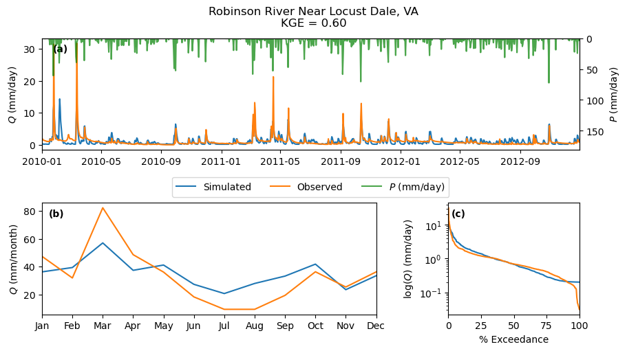
_ = gh.plot.signatures(
    discharge,
    clm_df.iloc[cal_idx:].prcp,
    title=f"{name}\nKGE = {kge:.2f}",
)