This page was generated from nlcd.ipynb. Interactive online version:

Land Use/Land Cover

from pathlib import Path

import matplotlib.pyplot as plt
import networkx as nx
import osmnx as ox

import pygeohydro as gh
from pynhd import NLDI

Land cover, imperviousness, and canopy data can be retrieved from the NLCD database. First, we use PyNHD to get the contributing watershed geometry of three NWIS stations with the ID of USGS-01031450, USGS-01031500, and USGS-01031510:

station_ids = ["01031450", "01318500", "01031510", "03460000"]
geometry = NLDI().get_basins(station_ids)
geometry.index = station_ids

We can now use the nlcd_bygeom and nlcd_bycoords functions to get the NLCD data.

Let’s start by nlcd_bygeom. This function has two positional arguments for passing the target geometries or points of interests and target resolution in meters. Note that, if a single geometry is passed and the geometry is not in EPSG:4326 CRS, geo_crs argument should be given as well. The second argument is the target resolution of the data in meters. The NLCD database is multi-resolution and based on the target resolution, the source data are resampled on the server side.

You should be mindful of the resolution since higher resolutions require more memory so if your requests requires more memory than the available memory on your system the code is likely to crash. You can either increase the resolution or divide your region of interest into smaller regions.

Moreover, the MRLC GeoServer has a limit of about 8 million pixels per request but PyGeoHydro takes care of the domain decomposition under-the-hood and divides the request to smaller requests then merges them. So the only bottleneck for requests is the amount of available memory on your system.

Both nlcd_bygeom and nlcd_bycoords functions can request for four layers from the MRLC web service; imperviousness, land use/land cover, impervious descriptors, and tree canopy. Since NLCD is released every couple of years, you can specify the target year via the years argument. Layers that are not included in this argument are ignored. By default, years is {'impervious': [2019], 'cover': [2019], 'canopy': [2019], 'descriptor': [2019]}.

Furthermore, we can specify the region of interest as well via the region argument. Valid values are L48 (for CONUS), HI (for Hawaii), AK (for Alaska), and PR (for Puerto Rico). By default, region is set to L48.

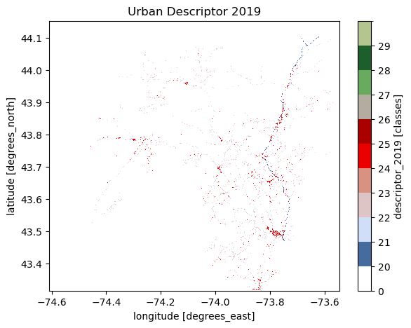
Let’s get the cover and impervious descriptor data at a 100 m resolution for all three stations

desc = gh.nlcd_bygeom(geometry, 100, years={"descriptor": 2019}, ssl=False)

This function returns a dict where its keys are the indices of the input GeoDataFrame.

cmap, norm, levels = gh.plot.descriptor_legends()

desc_2019 = desc["01318500"].descriptor_2019
ax = desc_2019.where(desc_2019 < 127).plot(
    size=5, cmap=cmap, levels=levels, cbar_kwargs={"ticks": levels[:-1]}
)
ax.axes.set_title("Urban Descriptor 2019")
ax.figure.savefig("_static/descriptor.png", bbox_inches="tight", facecolor="w")

Now let’s get the land cover data:

lulc = gh.nlcd_bygeom(geometry, 100, years={"cover": [2016, 2019]}, ssl=False)

Moreover, we can get the statistics of the cover data for each class or category:

stats = gh.cover_statistics(lulc["01318500"].cover_2019)
stats

Stats(classes={'Open Water': 3.218275304968691, 'Developed, Open Space': 1.6128251635756874, 'Developed, Low Intensity': 0.5524352553716665, 'Developed, Medium Intensity': 0.2678054930087095, 'Developed, High Intensity': 0.038027458129463905, 'Barren Land (Rock/Sand/Clay)': 0.0977190439205618, 'Deciduous Forest': 41.72741457073914, 'Evergreen Forest': 29.33253744552278, 'Mixed Forest': 14.194382537791228, 'Shrub-Forest': 0.692330207399452, 'Herbaceous-Forest': 0.33994242873308644, 'Shrub/Scrub': 0.05001186917632526, 'Grassland/Herbaceous': 0.18022710458933802, 'Pasture/Hay': 0.4438841476202877, 'Cultivated Crops': 0.008296899955519398, 'Woody Wetlands': 6.641437944950068, 'Emergent Herbaceous Wetlands': 0.6024471245479918}, categories={'Water': 3.218275304968691, 'Developed': 2.471093370085527, 'Barren': 0.0977190439205618, 'Forest': 86.28660719018569, 'Shrubland': 0.05001186917632526, 'Herbaceous': 0.18022710458933802, 'Planted/Cultivated': 0.4521810475758071, 'Wetlands': 7.24388506949806})

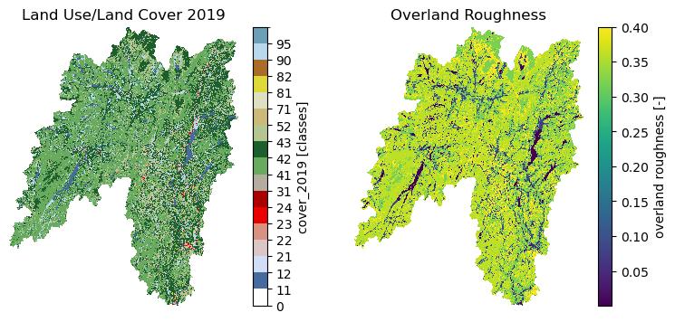
and an estimation of the overland roughness:

roughness = gh.overland_roughness(lulc["01318500"].cover_2019)

Additionally, PyGeoHydro provides a function for getting the official legends of the cover data. Let’s plot the data using this legends.

fig, (ax1, ax2) = plt.subplots(1, 2, figsize=(9, 4))

cmap, norm, levels = gh.plot.cover_legends()
cover = lulc["01318500"].cover_2019
cover.where(cover < 127).plot(ax=ax1, cmap=cmap, levels=levels, cbar_kwargs={"ticks": levels[:-1]})
ax1.set_title("Land Use/Land Cover 2019")
ax1.set_axis_off()

roughness.plot(ax=ax2)
ax2.set_title("Overland Roughness")
ax2.set_axis_off()
fig.savefig(Path("_static", "lulc.png"), bbox_inches="tight", facecolor="w")

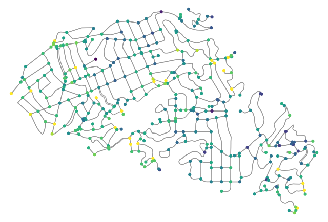
Now, let’s see nlcd_bycoords in action. The coordinates must be a list of (longitude, latitude) coordinates. Let’s use osmnx package to get a street network:

G = ox.graph_from_place("Piedmont, California, USA", network_type="drive")

Now, we can get land cover and tree canopy for each node based on their coordinates and then plot the results.

x, y = nx.get_node_attributes(G, "x").values(), nx.get_node_attributes(G, "y").values()
lulc = gh.nlcd_bycoords(list(zip(x, y)), years={"cover": [2019], "canopy": [2016]})
nx.set_node_attributes(G, dict(zip(G.nodes(), lulc.cover_2019)), "cover_2019")
nx.set_node_attributes(G, dict(zip(G.nodes(), lulc.canopy_2016)), "canopy_2016")

lulc.head()

	geometry	cover_2019	canopy_2016
0	POINT (-122.24760 37.82625)	23	27.0
1	POINT (-122.24719 37.82422)	22	21.0
2	POINT (-122.24611 37.82490)	23	20.0
3	POINT (-122.24534 37.82541)	23	24.0
4	POINT (-122.24447 37.82595)	23	25.0

nc = ox.plot.get_node_colors_by_attr(G, "canopy_2016", cmap="viridis_r")
fig, ax = ox.plot_graph(
    G,
    node_color=nc,
    node_size=20,
    save=True,
    bgcolor="w",
)

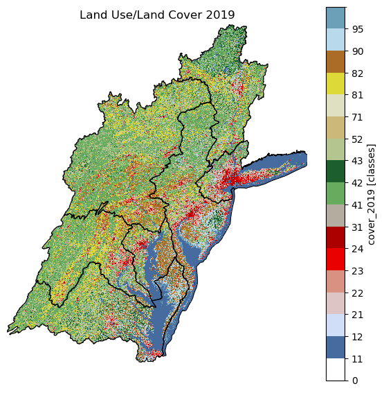
Next, let’s get the data for a larger area at a coarser resolution. For example, we get the Upper Hudson subregion boundary using pygeohydro.WBD, then get the cover data within the area.

wbd = gh.WBD("huc4")
hud = wbd.byids("huc4", ["0202", "0203", "0204", "0205", "0206", "0207", "0208"])
hud = hud.set_index("huc4")
lulc = gh.nlcd_bygeom(hud, 1000, years={"cover": [2019]})

cmap, norm, levels = gh.plot.cover_legends()
fig, ax = plt.subplots(1, 1, figsize=(7, 7))
xmin, ymin, xmax, ymax = hud.unary_union.bounds

cover = {h: da.cover_2019.where(da.cover_2019 < 127) for h, da in lulc.items()}

cover["0202"].plot(ax=ax, cmap=cmap, levels=levels, cbar_kwargs={"ticks": levels[:-1]})
_ = cover.pop("0202")
for da in cover.values():
    da.plot(ax=ax, cmap=cmap, levels=levels, add_colorbar=False)
hud.plot(ax=ax, facecolor="none", edgecolor="k", linewidth=0.8)
ax.set_xlim(xmin, xmax)
ax.set_ylim(ymin, ymax)
ax.set_axis_off()
ax.set_title("Land Use/Land Cover 2019")
ax.margins(0)