This page was generated from nldas.ipynb. Interactive online version:

NLDAS2 Forcing

from __future__ import annotations

from pathlib import Path

import pynldas2 as nldas
from pygeohydro import WBD

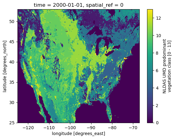
The NLDAS2 database provides forcing data at 1/8th-degree grid spacing and range from 01 Jan 1979 to present. Let’s take a look at NLDAS2 grid mask that includes land, water, soil, and vegetation masks:

grid = nldas.get_grid_mask()
grid

<xarray.Dataset> Size: 2MB
Dimensions:      (lon: 464, lat: 224, time: 1, bnds: 2)
Coordinates:
  * lon          (lon) float32 2kB -124.9 -124.8 -124.7 ... -67.31 -67.19 -67.06
  * lat          (lat) float32 896B 25.06 25.19 25.31 ... 52.69 52.81 52.94
  * time         (time) datetime64[ns] 8B 2000-01-01
    spatial_ref  int64 8B 0
Dimensions without coordinates: bnds
Data variables:
    time_bnds    (time, bnds) datetime64[ns] 16B ...
    NLDAS_mask   (time, lat, lon) float32 416kB ...
    CONUS_mask   (time, lat, lon) float32 416kB ...
    NLDAS_veg    (time, lat, lon) float32 416kB ...
    NLDAS_soil   (time, lat, lon) float32 416kB ...
Attributes: (12/13)
    missing_value:          -9999.0
    time_definition:        constant
    title:                  NLDAS masks and predominant vegetation/soil
    institution:            NASA GSFC
    history:                created on date: Fri Mar  8 15:58:50 2019
    references:             Mitchell_etal_JGR_2004; Xia_etal_JGR_2012
    ...                     ...
    website:                https://ldas.gsfc.nasa.gov/nldas/
    MAP_PROJECTION:         EQUIDISTANT CYLINDRICAL
    SOUTH_WEST_CORNER_LAT:  25.0625
    SOUTH_WEST_CORNER_LON:  -124.9375
    DX:                     0.125
    DY:                     0.125

xarray.Dataset

• Dimensions:
  • lon: 464
  • lat: 224
  • time: 1
  • bnds: 2
• Coordinates: (4)
  • lon
    (lon)
    float32
    -124.9 -124.8 ... -67.19 -67.06

    units :

    degrees_east

    standard_name :

    longitude

    long_name :

    longitude

    vmin :

    -124.9375

    vmax :

    -67.0625

    axis :

    X

    array([-124.9375, -124.8125, -124.6875, ...,  -67.3125,  -67.1875,  -67.0625],
          dtype=float32)

  • lat
    (lat)
    float32
    25.06 25.19 25.31 ... 52.81 52.94

    units :

    degrees_north

    standard_name :

    latitude

    long_name :

    latitude

    vmin :

    25.0625

    vmax :

    52.9375

    axis :

    Y

    array([25.0625, 25.1875, 25.3125, ..., 52.6875, 52.8125, 52.9375],
          dtype=float32)

  • time
    (time)
    datetime64[ns]
    2000-01-01

    long_name :

    time

    time_increment :

    1

    bounds :

    time_bnds

    array(['2000-01-01T00:00:00.000000000'], dtype='datetime64[ns]')

  • spatial_ref
    ()
    int64
    0

    crs_wkt :

    GEOGCS["WGS 84",DATUM["WGS_1984",SPHEROID["WGS 84",6378137,298.257223563,AUTHORITY["EPSG","7030"]],AUTHORITY["EPSG","6326"]],PRIMEM["Greenwich",0,AUTHORITY["EPSG","8901"]],UNIT["degree",0.0174532925199433,AUTHORITY["EPSG","9122"]],AXIS["Latitude",NORTH],AXIS["Longitude",EAST],AUTHORITY["EPSG","4326"]]

    semi_major_axis :

    6378137.0

    semi_minor_axis :

    6356752.314245179

    inverse_flattening :

    298.257223563

    reference_ellipsoid_name :

    WGS 84

    longitude_of_prime_meridian :

    0.0

    prime_meridian_name :

    Greenwich

    geographic_crs_name :

    WGS 84

    horizontal_datum_name :

    World Geodetic System 1984

    grid_mapping_name :

    latitude_longitude

    spatial_ref :

    GEOGCS["WGS 84",DATUM["WGS_1984",SPHEROID["WGS 84",6378137,298.257223563,AUTHORITY["EPSG","7030"]],AUTHORITY["EPSG","6326"]],PRIMEM["Greenwich",0,AUTHORITY["EPSG","8901"]],UNIT["degree",0.0174532925199433,AUTHORITY["EPSG","9122"]],AXIS["Latitude",NORTH],AXIS["Longitude",EAST],AUTHORITY["EPSG","4326"]]

    GeoTransform :

    -125.0 0.125 0.0 25.0 0.0 0.125

    array(0)

• Data variables: (5)
  • time_bnds
    (time, bnds)
    datetime64[ns]
    ...

    [2 values with dtype=datetime64[ns]]

  • NLDAS_mask
    (time, lat, lon)
    float32
    ...

    units :

    0 = water; 1 = land

    standard_name :

    land mask

    long_name :

    NLDAS UMD unified land mask

    cell_methods :

    time: mean

    vmin :

    0.0

    vmax :

    1.0

    [103936 values with dtype=float32]

  • CONUS_mask
    (time, lat, lon)
    float32
    ...

    units :

    0 = water; 1 = land

    standard_name :

    CONUS mask

    long_name :

    NLDAS CONUS mask

    cell_methods :

    time: mean

    vmin :

    0.0

    vmax :

    1.0

    [103936 values with dtype=float32]

  • NLDAS_veg
    (time, lat, lon)
    float32
    ...

    units :

    0 - 13

    standard_name :

    vegetation class

    long_name :

    NLDAS UMD predominant vegetation class

    cell_methods :

    time: mean

    vmin :

    0.0

    vmax :

    13.0

    [103936 values with dtype=float32]

  • NLDAS_soil
    (time, lat, lon)
    float32
    ...

    units :

    0 - 14

    standard_name :

    soil texture type

    long_name :

    NLDAS STATSGO predominant soil texture type

    cell_methods :

    time: mean

    vmin :

    0.0

    vmax :

    14.0

    [103936 values with dtype=float32]

• Indexes: (3)
  • lon
    PandasIndex

    PandasIndex(Index([-124.9375, -124.8125, -124.6875, -124.5625, -124.4375, -124.3125,
           -124.1875, -124.0625, -123.9375, -123.8125,
           ...
            -68.1875,  -68.0625,  -67.9375,  -67.8125,  -67.6875,  -67.5625,
            -67.4375,  -67.3125,  -67.1875,  -67.0625],
          dtype='float32', name='lon', length=464))

  • lat
    PandasIndex

    PandasIndex(Index([25.0625, 25.1875, 25.3125, 25.4375, 25.5625, 25.6875, 25.8125, 25.9375,
           26.0625, 26.1875,
           ...
           51.8125, 51.9375, 52.0625, 52.1875, 52.3125, 52.4375, 52.5625, 52.6875,
           52.8125, 52.9375],
          dtype='float32', name='lat', length=224))

  • time
    PandasIndex

    PandasIndex(DatetimeIndex(['2000-01-01'], dtype='datetime64[ns]', name='time', freq=None))

• Attributes: (13)

  missing_value :

  -9999.0

  time_definition :

  constant

  title :

  NLDAS masks and predominant vegetation/soil

  institution :

  NASA GSFC

  history :

  created on date: Fri Mar 8 15:58:50 2019

  references :

  Mitchell_etal_JGR_2004; Xia_etal_JGR_2012

  conventions :

  CF-1.6

  website :

  https://ldas.gsfc.nasa.gov/nldas/

  MAP_PROJECTION :

  EQUIDISTANT CYLINDRICAL

  SOUTH_WEST_CORNER_LAT :

  25.0625

  SOUTH_WEST_CORNER_LON :

  -124.9375

  DX :

  0.125

  DY :

  0.125

For example, let’s plot the vegetation mask.

ax = grid.NLDAS_veg.plot()
ax.figure.savefig(Path("_static", "nldas_grid.png"), facecolor="w", bbox_inches="tight")

Next, we use PyGeoHydro to get the geometry of a HUC8 with ID of 1306003:

huc8 = WBD("huc8")
geometry = huc8.byids("huc8", "13060003").geometry.iloc[0]

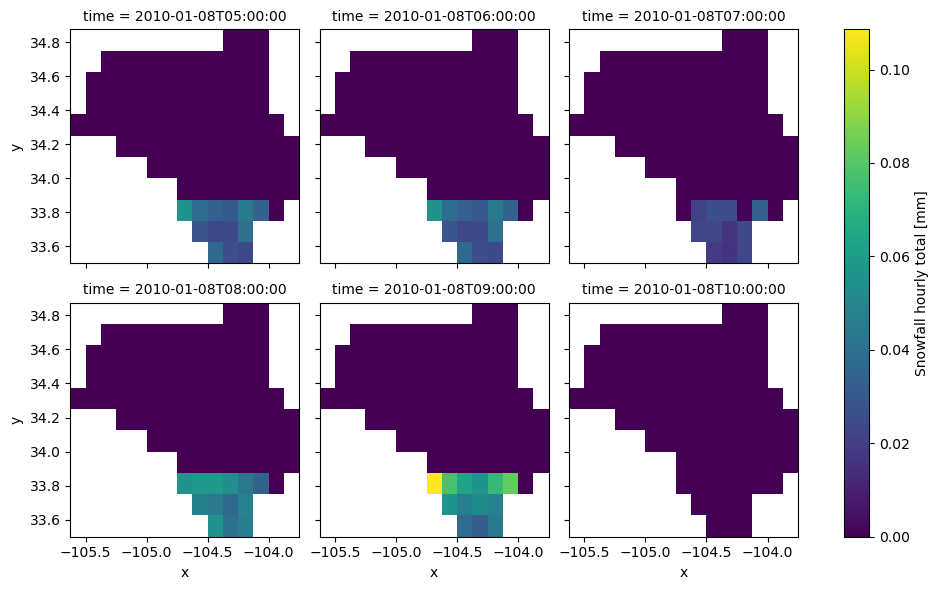
PyNLDAS2 allows us to get the data for a list of coordinates using pynldas2.get_bycoords or for a region as gridded data using pynldas2.get_bygeom. Here, we use the latter. Note that if we don’t pass any variables, all variables will be downloaded. Additionally, we can pass snow=True to separate snow portion of precipitation using temperature. PyNLDAS2 provides access to NLDAS2 data from two sources: grib and netcdf. They are mostly similar so if for some reason one of the sources is not temporarly available, you can use the other one. The default source is grib.

clm = nldas.get_bygeom(geometry, "2010-01-08", "2010-01-08", 4326, variables="prcp", snow=True)

ax = clm.snow.sel(time=slice("2010-01-08T05:00:00", "2010-01-08T010:00:00")).plot(
    col="time", col_wrap=3
)
ax.fig.savefig(Path("_static", "nldas_snow.png"), facecolor="w", bbox_inches="tight")