This page was generated from nwis.ipynb. Interactive online version:

River Discharge

import pandas as pd
import xarray as xr

import pydaymet as daymet
import pygeohydro as gh
from pygeohydro import NWIS, plot

_ = xr.set_options(display_expand_attrs=False)

We can explore the available NWIS stations within a bounding box using interactive_map function. It returns an interactive map and by clicking on an station some of the most important properties of stations are shown so you can decide which station(s) to choose from.

bbox = (-69.5, 45, -69, 45.5)

nwis_kwds = {"hasDataTypeCd": "dv", "outputDataTypeCd": "dv", "parameterCd": "00060"}
gh.interactive_map(bbox, nwis_kwds=nwis_kwds)

Make this Notebook Trusted to load map: File -> Trust Notebook

We can get more information about these stations using the get_info function from NWIS class.

nwis = NWIS()
query = {
    "bBox": ",".join(f"{b:.06f}" for b in bbox),
    "hasDataTypeCd": "dv",
    "outputDataTypeCd": "dv",
}
info_box = nwis.get_info(query)

Now, let’s select all the stations that their daily mean streamflow data are available between 2000-01-01 and 2010-12-31.

dates = ("2000-01-01", "2010-12-31")
stations = info_box[
    (info_box.begin_date <= dates[0]) & (info_box.end_date >= dates[1])
].site_no.tolist()

One of the useful information in the database in Hydro-Climatic Data Network - 2009 (HCDN-2009) flag. This flag shows whether the station is natural (True) or affected by human activities (False). If an station is not available in the HCDN dataset None is returned.

query = {
    "site": ",".join(stations),
    "hasDataTypeCd": "dv",
    "outputDataTypeCd": "dv",
}
info = nwis.get_info(query, expanded=True)
info.set_index("site_no").hcdn_2009

site_no
01031450           False
01031500            True
01031500            True
01031500            True
01031500            True
01033000           False
451031069185301    False
451105069270801    False
Name: hcdn_2009, dtype: bool

We can get the daily mean streamflow for these stations using the get_streamflow function. This function has a flag to return the data mm/day rather than the default cms which is useful for hydrolgy models and plotting hydrologic signatures.

qobs = nwis.get_streamflow(stations, dates, mmd=True)

/var/folders/jx/s06wj7hs325c_2yd2g5209sr0000gp/T/ipykernel_90548/3705647618.py:1: UserWarning: Dropped 1 stations since they don't have discharge data from 2000-01-01 to 2010-12-31.
  qobs = nwis.get_streamflow(stations, dates, mmd=True)

By default, get_streamflow returns a pandas.DataFrame that has an attrs method containing metadata for all the stations.

Moreover, we can get the same data as xarray.Dataset as follows:

qobs_ds = nwis.get_streamflow(stations, dates, mmd=True, to_xarray=True)
qobs_ds

/var/folders/jx/s06wj7hs325c_2yd2g5209sr0000gp/T/ipykernel_90548/3292066144.py:1: UserWarning: Dropped 1 stations since they don't have discharge data from 2000-01-01 to 2010-12-31.
  qobs_ds = nwis.get_streamflow(stations, dates, mmd=True, to_xarray=True)

<xarray.Dataset>
Dimensions:       (time: 4018, station_id: 2)
Coordinates:
  * time          (time) datetime64[ns] 2000-01-01T05:00:00 ... 2010-12-31T05...
  * station_id    (station_id) object 'USGS-01031450' 'USGS-01031500'
Data variables:
    discharge     (time, station_id) float64 0.7128 0.667 0.6435 ... 1.534 1.407
    station_nm    (station_id) <U44 'Kingsbury Stream At Abbot Village, Maine...
    dec_lat_va    (station_id) float64 45.18 45.17
    dec_long_va   (station_id) float64 -69.45 -69.31
    alt_va        (station_id) float64 423.0 358.5
    alt_acy_va    (station_id) float64 0.01 0.01
    alt_datum_cd  (station_id) <U6 'NGVD29' 'NGVD29'
    huc_cd        (station_id) <U8 '01020004' '01020004'
    begin_date    (station_id) <U10 '1997-07-26' '1902-10-01'
    end_date      (station_id) <U10 '2023-11-26' '2023-11-26'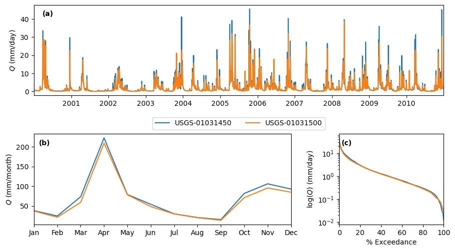
Attributes: (1)

xarray.Dataset

• Dimensions:
  • time: 4018
  • station_id: 2
• Coordinates: (2)
  • time
    (time)
    datetime64[ns]
    2000-01-01T05:00:00 ... 2010-12-...

    array(['2000-01-01T05:00:00.000000000', '2000-01-02T05:00:00.000000000',
           '2000-01-03T05:00:00.000000000', ..., '2010-12-29T05:00:00.000000000',
           '2010-12-30T05:00:00.000000000', '2010-12-31T05:00:00.000000000'],
          dtype='datetime64[ns]')

  • station_id
    (station_id)
    object
    'USGS-01031450' 'USGS-01031500'

    array(['USGS-01031450', 'USGS-01031500'], dtype=object)

• Data variables: (10)
  • discharge
    (time, station_id)
    float64
    0.7128 0.667 0.6435 ... 1.534 1.407

    units :

    mm/day

    array([[0.7127834 , 0.66699154],
           [0.64348501, 0.62589727],
           [0.59398616, 0.5911252 ],
           ...,
           [1.61366241, 1.55842099],
           [1.53446425, 1.46358807],
           [1.53446425, 1.40668832]])

  • station_nm
    (station_id)
    <U44
    'Kingsbury Stream At Abbot Villa...

    long_name :

    station name

    array(['Kingsbury Stream At Abbot Village, Maine',
           'Piscataquis River Near Dover-Foxcroft, Maine'], dtype='<U44')

  • dec_lat_va
    (station_id)
    float64
    45.18 45.17

    long_name :

    latitude

    units :

    decimal_degrees

    array([45.1844444, 45.175    ])

  • dec_long_va
    (station_id)
    float64
    -69.45 -69.31

    long_name :

    longitude

    units :

    decimal_degrees

    array([-69.4522222, -69.3147222])

  • alt_va
    (station_id)
    float64
    423.0 358.5

    long_name :

    altitude

    units :

    ft

    array([423.  , 358.47])

  • alt_acy_va
    (station_id)
    float64
    0.01 0.01

    long_name :

    altitude accuracy

    array([0.01, 0.01])

  • alt_datum_cd
    (station_id)
    <U6
    'NGVD29' 'NGVD29'

    long_name :

    altitude datum

    array(['NGVD29', 'NGVD29'], dtype='<U6')

  • huc_cd
    (station_id)
    <U8
    '01020004' '01020004'

    long_name :

    hydrologic unit code

    array(['01020004', '01020004'], dtype='<U8')

  • begin_date
    (station_id)
    <U10
    '1997-07-26' '1902-10-01'

    long_name :

    availability begin date

    array(['1997-07-26', '1902-10-01'], dtype='<U10')

  • end_date
    (station_id)
    <U10
    '2023-11-26' '2023-11-26'

    long_name :

    availability end date

    array(['2023-11-26', '2023-11-26'], dtype='<U10')

• Indexes: (2)
  • time
    PandasIndex

    PandasIndex(DatetimeIndex(['2000-01-01 05:00:00', '2000-01-02 05:00:00',
                   '2000-01-03 05:00:00', '2000-01-04 05:00:00',
                   '2000-01-05 05:00:00', '2000-01-06 05:00:00',
                   '2000-01-07 05:00:00', '2000-01-08 05:00:00',
                   '2000-01-09 05:00:00', '2000-01-10 05:00:00',
                   ...
                   '2010-12-22 05:00:00', '2010-12-23 05:00:00',
                   '2010-12-24 05:00:00', '2010-12-25 05:00:00',
                   '2010-12-26 05:00:00', '2010-12-27 05:00:00',
                   '2010-12-28 05:00:00', '2010-12-29 05:00:00',
                   '2010-12-30 05:00:00', '2010-12-31 05:00:00'],
                  dtype='datetime64[ns]', name='time', length=4018, freq=None))

  • station_id
    PandasIndex

    PandasIndex(Index(['USGS-01031450', 'USGS-01031500'], dtype='object', name='station_id'))

• Attributes: (1)

  tz :

  UTC

Then we can use the signatures function to plot hydrologic signatures of the streamflow. Note that the input time series should be in mm/day. This function has argument, output, for saving the plot as a png file.

plot.signatures(qobs, output="_static/example_plots_signatures.png")

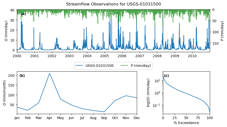
This function also can show precipitation data as a bar plot. Let’s use PyDaymet to get the precipitation at the NWIS stations location.

sid = "01031500"
coords = tuple(info[info.site_no == sid][["dec_long_va", "dec_lat_va"]].to_numpy()[0])
prcp = daymet.get_bycoords(coords, dates, variables="prcp", ssl=False)
qobs.index = pd.to_datetime(qobs.index.strftime("%Y-%m-%d"))

plot.signatures(
    qobs[f"USGS-{sid}"],
    prcp,
    title=f"Streamflow Observations for USGS-{sid}",
    output="_static/nwis.png",
)

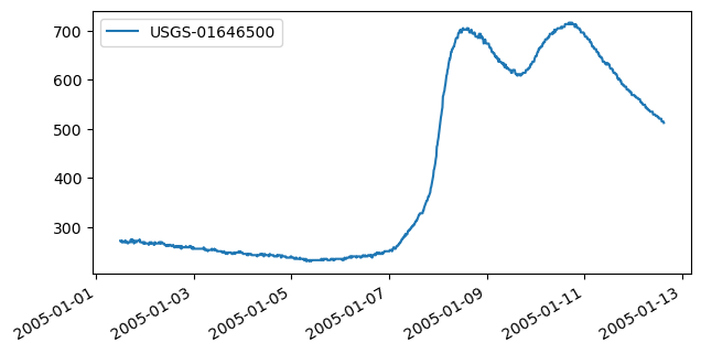
We can also get instantaneous streamflow data using get_streamflow. This method assumes that the input dates are in UTC time zone and returns the data in UTC time zone as well.

qobs = nwis.get_streamflow("01646500", ("2005-01-01 12:00", "2005-01-12 15:00"), freq="iv")
_ = qobs.plot(figsize=(7, 3.5))