Querying the Water Data API
WaterData queries the USGS Water Data API. It sends the key in USGS_API_KEY, when set, in
the X-Api-Key header. This notebook asks for the monitoring locations in a box around
Washington, DC, streams the pages as they arrive, collects a QueryResult, narrows the
query with a CQL2 filter, and fetches daily discharge split by year. to_arrow() turns
each result into a table for geopandas or polars, which needs the arrow extra.
A service keeps its HTTP connections open until it is closed. In a script, use it in
a with block, with WaterData() as wd:, which closes it on exit. A notebook keeps one
service across cells, so it calls wd.close() explicitly in its last cell.
Stream pages
iter_pages() yields one Page per response and follows each page's next link. A
limit of 200 shows the paging; the default is 10,000 features a page. WaterData reports no
numberMatched, so the total is known only once the last page arrives.
for page in wd.iter_pages("monitoring-locations", bbox=DC, params={"limit": "200"}):
    print(page.status, page.feature_count, page.number_matched)
200 200 None
200 112 None
Collect a result
collect() gathers every page into one FeatureCollection and records how the traversal
went: the checks that passed and the CRS the server named.
sites = wd.collect("monitoring-locations", bbox=DC)
print(len(sites.geojson["features"]), "features in", sites.pagination.page_count, "page(s)")
print(sites.pagination.completeness, sites.pagination.checks)
print(sites.crs.effective, sites.crs.source)
312 features in 1 page(s)
complete ('end_of_links', 'unique_ids')
http://www.opengis.net/def/crs/OGC/1.3/CRS84 content_crs
Filter with CQL2
A CQL2-Text filter combines with the bounding box. Only the stream sites:
streams = wd.collect("monitoring-locations", bbox=DC, filter="site_type_code = 'ST'")
for feature in streams.geojson["features"][:10]:
    print(feature["id"], feature["properties"]["monitoring_location_name"])
USEPA-385353076573301 DC90S001
USGS-01646550 LITTLE FALLS BRANCH NEAR BETHESDA, MD
USGS-01646563 MILL CREEK TRIB NR DALECARLIA RES AT WASHINGTON DC
USGS-01646564 MILL CREEK AT DALECARLIA RES NEAR CHEVY CHASE, MD
USGS-01646565 EAST CREEK NR DALECARLIA RES AT WASHINGTON, DC
USGS-0164656550 EAST CREEK TRIB NR DALECARLIA RES AT WASHINGTON DC
USGS-01646566 EAST CREEK AT DALECARLIA RES AT WASHINGTON, DC
USGS-01646567 EAST CREEK AT DALECARLIA RES NEAR CHEVY CHASE, MD
USGS-01646568 MILL CREEK AT DALECARLIA RES NEAR BETHESDA, MD
USGS-01646569 MILL CREEK AT DALECARLIA RES AT BROOKMONT, MD
Map the sites
to_arrow() returns a pyarrow Table whose geometry column carries the CRS, so
geopandas reads it as a GeoDataFrame with that CRS.
import geopandas as gpd

frame = gpd.GeoDataFrame.from_arrow(sites.to_arrow())
print(frame.crs)
frame["site_type"].value_counts().head()
{"$schema": "https://proj.org/schemas/v0.7/projjson.schema.json", "type": "GeographicCRS", "name": "WGS 84 (CRS84)", "datum_ensemble": {"name": "World Geodetic System 1984 ensemble", "members": [{"name": "World Geodetic System 1984 (Transit)", "id": {"authority": "EPSG", "code": 1166}}, {"name": "World Geodetic System 1984 (G730)", "id": {"authority": "EPSG", "code": 1152}}, {"name": "World Geodetic System 1984 (G873)", "id": {"authority": "EPSG", "code": 1153}}, {"name": "World Geodetic System 1984 (G1150)", "id": {"authority": "EPSG", "code": 1154}}, {"name": "World Geodetic System 1984 (G1674)", "id": {"authority": "EPSG", "code": 1155}}, {"name": "World Geodetic System 1984 (G1762)", "id": {"authority": "EPSG", "code": 1156}}, {"name": "World Geodetic System 1984 (G2139)", "id": {"authority": "EPSG", "code": 1309}}, {"name": "World Geodetic System 1984 (G2296)", "id": {"authority": "EPSG", "code": 1383}}], "ellipsoid": {"name": "WGS 84", "semi_major_axis": 6378137, "inverse_flattening": 298.257223563}, "accuracy": "2.0", "id": {"authority": "EPSG", "code": 6326}}, "coordinate_system": {"subtype": "ellipsoidal", "axis": [{"name": "Geodetic longitude", "abbreviation": "Lon", "direction": "east", "unit": "degree"}, {"name": "Geodetic latitude", "abbreviation": "Lat", "direction": "north", "unit": "degree"}]}, "scope": "Not known.", "area": "World.", "bbox": {"south_latitude": -90, "west_longitude": -180, "north_latitude": 90, "east_longitude": 180}, "id": {"authority": "OGC", "code": "CRS84"}}


site_type
Well                             120
Stream                           114
Estuary                           17
Tidal stream                      17
Collector or Ranney type well     11
Name: count, dtype: int64
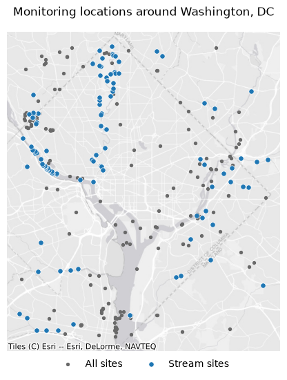
contextily draws a basemap under the points. Its tiles are in Web Mercator (EPSG:3857), so both layers are reprojected to it first.
import contextily as ctx
from xyzservices import providers

ax = frame.to_crs(3857).plot(color="dimgray", markersize=8, figsize=(6, 6), label="All sites")
gpd.GeoDataFrame.from_arrow(streams.to_arrow()).to_crs(3857).plot(
    ax=ax, color="tab:blue", edgecolor="white", linewidth=0.5, markersize=28, label="Stream sites"
)
ctx.add_basemap(ax, source=providers.Esri.WorldGrayCanvas)
ax.legend(loc="upper center", bbox_to_anchor=(0.5, 0), ncols=2, frameon=False)
ax.set(title="Monitoring locations around Washington, DC")
ax.set_axis_off()
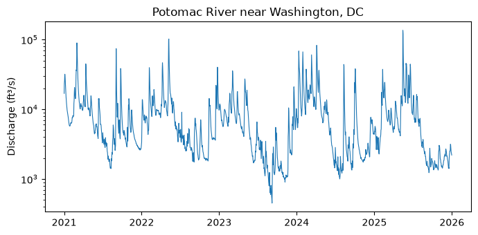
Daily discharge, split by year
split_datetime="year" splits the interval into one piece a year and runs the pieces
concurrently, as USGS's efficiency guidance recommends. Parameter 00060 is discharge
and statistic 00003 the daily mean.
daily = wd.collect(
    "daily",
    params={
        "monitoring_location_id": "USGS-01646500",
        "parameter_code": "00060",
        "statistic_id": "00003",
        "datetime": "2021-01-01/2025-12-31",
    },
    split_datetime="year",
)
print(len(daily.geojson["features"]), "days in", daily.pagination.page_count, "pages")
print(daily.pagination.completeness, daily.pagination.checks)
1826 days in 5 pages
complete ('end_of_links', 'unique_ids')
polars reads the same table. The pieces arrive in the order they finish, so sort by date before plotting.
import polars as pl

values = (
    pl.DataFrame(daily.to_arrow())
    .select(pl.col("time").str.to_date(), pl.col("value").cast(pl.Float64))
    .sort("time")
)
values.head()
| time | value |
|---|---|
| date | f64 |
| 2021-01-01 | 16900.0 |
| 2021-01-02 | 23400.0 |
| 2021-01-03 | 25700.0 |
| 2021-01-04 | 31900.0 |
| 2021-01-05 | 31500.0 |
import matplotlib.pyplot as plt

fig, ax = plt.subplots(figsize=(7, 3.5))
ax.plot(values["time"], values["value"], linewidth=0.8)
ax.set(yscale="log", ylabel="Discharge (ft³/s)", title="Potomac River near Washington, DC")
fig.tight_layout()