Querying FabricData
FabricData queries the USGS Geospatial Fabric service. It takes no key and never
receives USGS_API_KEY. This notebook looks up the service's collections and the
properties of gagesii, the GAGES-II streamgages, then collects the gages in a box
around Washington, DC, narrows the query with a CQL2 filter, and maps the result.
to_arrow() turns a result into a table for geopandas, which needs the arrow extra.
A service keeps its HTTP connections open until it is closed. In a script, use it in
a with block, with FabricData() as fabric:, which closes it on exit. A notebook keeps one
service across cells, so it calls fabric.close() explicitly in its last cell.
Look at the collection
collections() returns the index and queryables() the properties of one collection
that a query can name. Both are cached for an hour. Each query checks its collection
and parameter names against that cache first, so a typo raises an error that lists the
valid names.
ids = [collection.id for collection in fabric.collections().collections or ()]
print(len(ids), "collections:", ", ".join(ids[:6]), "...")
31 collections: catchmentsp, nhdarea, nhdflowline_network, nhdflowline_nonnetwork, nhdwaterbody, gagesii ...
for name, prop in (fabric.queryables("gagesii").properties or {}).items():
    print(f"{name:12} {prop.type or prop.format}")
geometry     geometry-any
ogc_fid      integer
id           string
staid        string
staname      string
class        string
aggecoregi   string
drain_sqkm   number
huc02        string
lat_gage     number
lng_gage     number
state        string
hcdn_2009    string
active09     string
flyrs1900    integer
flyrs1950    integer
flyrs1990    integer
Collect the gages in a box
collect() gathers every page into one FeatureCollection and records how the traversal
went: the checks that passed and the CRS the server named. FabricData reports
numberMatched, so the count check compares it with the features received. It sends
X-RateLimit-* headers on every response, which the client uses to space its requests.
gages = fabric.collect("gagesii", bbox=DC)
print(len(gages.geojson["features"]), "gages in", gages.pagination.page_count, "page(s)")
print(gages.pagination.completeness, gages.pagination.checks)
print(gages.crs.effective, gages.crs.source)
print("X-RateLimit-Limit:", gages.pages[0].headers["x-ratelimit-limit"])
8 gages in 1 page(s)
complete ('end_of_links', 'count', 'unique_ids')
http://www.opengis.net/def/crs/OGC/1.3/CRS84 content_crs
X-RateLimit-Limit: 300
Filter with CQL2
A CQL2-Text filter combines with the bounding box. Only the gages that drain more
than 100 km²:
large = fabric.collect("gagesii", bbox=DC, filter="drain_sqkm > 100")
for feature in large.geojson["features"]:
    props = feature["properties"]
    print(feature["id"], props["staname"], props["drain_sqkm"])
01648000 ROCK CREEK AT SHERRILL DRIVE WASHINGTON, DC 136.8279
01649500 NORTH EAST BRANCH ANACOSTIA RIVER AT RIVERDALE, MD 188.0622
01651000 NW BRANCH ANACOSTIA RIVER NEAR HYATTSVILLE, MD 127.8054
Read the gages with geopandas
to_arrow() returns a pyarrow Table whose geometry column carries the CRS, so
geopandas reads it as a GeoDataFrame with that CRS. Each gage is a MultiPoint of one
point.
import geopandas as gpd

frame = gpd.GeoDataFrame.from_arrow(gages.to_arrow())
print(frame.crs)
frame.sort_values("staid")[["staid", "staname", "state", "drain_sqkm"]]
{"$schema": "https://proj.org/schemas/v0.7/projjson.schema.json", "type": "GeographicCRS", "name": "WGS 84 (CRS84)", "datum_ensemble": {"name": "World Geodetic System 1984 ensemble", "members": [{"name": "World Geodetic System 1984 (Transit)", "id": {"authority": "EPSG", "code": 1166}}, {"name": "World Geodetic System 1984 (G730)", "id": {"authority": "EPSG", "code": 1152}}, {"name": "World Geodetic System 1984 (G873)", "id": {"authority": "EPSG", "code": 1153}}, {"name": "World Geodetic System 1984 (G1150)", "id": {"authority": "EPSG", "code": 1154}}, {"name": "World Geodetic System 1984 (G1674)", "id": {"authority": "EPSG", "code": 1155}}, {"name": "World Geodetic System 1984 (G1762)", "id": {"authority": "EPSG", "code": 1156}}, {"name": "World Geodetic System 1984 (G2139)", "id": {"authority": "EPSG", "code": 1309}}, {"name": "World Geodetic System 1984 (G2296)", "id": {"authority": "EPSG", "code": 1383}}], "ellipsoid": {"name": "WGS 84", "semi_major_axis": 6378137, "inverse_flattening": 298.257223563}, "accuracy": "2.0", "id": {"authority": "EPSG", "code": 6326}}, "coordinate_system": {"subtype": "ellipsoidal", "axis": [{"name": "Geodetic longitude", "abbreviation": "Lon", "direction": "east", "unit": "degree"}, {"name": "Geodetic latitude", "abbreviation": "Lat", "direction": "north", "unit": "degree"}]}, "scope": "Not known.", "area": "World.", "bbox": {"south_latitude": -90, "west_longitude": -180, "north_latitude": 90, "east_longitude": 180}, "id": {"authority": "OGC", "code": "CRS84"}}
| staid | staname | state | drain_sqkm | |
|---|---|---|---|---|
| 0 | 01646550 | LITTLE FALLS BRANCH NEAR BETHESDA, MD | MD | 10.5219 |
| 1 | 01648000 | ROCK CREEK AT SHERRILL DRIVE WASHINGTON, DC | DC | 136.8279 |
| 2 | 01649500 | NORTH EAST BRANCH ANACOSTIA RIVER AT RIVERDALE... | MD | 188.0622 |
| 3 | 01650800 | SLIGO CREEK NEAR TAKOMA PARK, MD | MD | 16.7013 |
| 4 | 01651000 | NW BRANCH ANACOSTIA RIVER NEAR HYATTSVILLE, MD | MD | 127.8054 |
| 5 | 01651800 | WATTS BRANCH AT WASHINGTON, DC | DC | 8.5590 |
| 6 | 01652500 | FOURMILE RUN AT ALEXANDRIA, VA | VA | 34.5501 |
| 7 | 01653000 | CAMERON RUN AT ALEXANDRIA, VA | VA | 87.3063 |
Map the gages
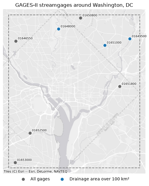
The dashed rectangle is the query's bounding box. contextily draws a basemap under the gages; its tiles are in Web Mercator (EPSG:3857), so every layer is reprojected to it.
import contextily as ctx
import matplotlib.patheffects as pe
import matplotlib.pyplot as plt
import shapely
from xyzservices import providers

points = frame.to_crs(3857)
big = gpd.GeoDataFrame.from_arrow(large.to_arrow()).to_crs(3857)
box = gpd.GeoSeries([shapely.box(*DC)], crs=frame.crs).to_crs(3857)
ax = points.plot(color="dimgray", markersize=40, figsize=(6, 6.5), label="All gages")
big.plot(
    ax=ax,
    color="tab:blue",
    edgecolor="white",
    markersize=70,
    label="Drainage area over 100 km²",
)
halo = [pe.withStroke(linewidth=2.5, foreground="white")]
for geometry, staid in zip(points.geometry, points["staid"], strict=True):
    x, y = geometry.centroid.coords[0]
    ax.annotate(
        staid, (x, y), xytext=(5, 4), textcoords="offset points", fontsize=7, path_effects=halo
    )
box.boundary.plot(ax=ax, color="gray", linestyle="--")
west, south, east, north = box.total_bounds
ax.set_xlim(west - 1000, east + 1000)  # meters
ax.set_ylim(south - 1000, north + 1000)
ctx.add_basemap(ax, source=providers.Esri.WorldGrayCanvas)
ax.legend(loc="upper center", bbox_to_anchor=(0.5, 0), ncols=2, frameon=False)
ax.set(title="GAGES-II streamgages around Washington, DC")
ax.set_axis_off()
plt.tight_layout()