Querying GeoConnex
GeoConnex queries the reference features at reference.geoconnex.us. It takes no key
and never receives USGS_API_KEY. This notebook lists the 22 two-digit hydrologic
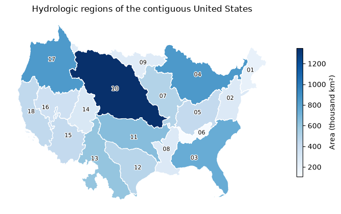
regions of hu02 without their geometry, streams them a few at a time, and maps the 18
regions of the contiguous United States with a CQL2 filter. to_arrow() turns each
result into a table for polars or geopandas, which needs the arrow extra.
A service keeps its HTTP connections open until it is closed. In a script, use it in
a with block, with GeoConnex() as gc:, which closes it on exit. A notebook keeps one
service across cells, so it calls gc.close() explicitly in its last cell.
List the regions
Geometry is most of a response. skipGeometry asks the server to leave it out, and
keep_pages=True keeps each page's bytes in Page.content, so the notebook can report
their size. to_arrow() on features without geometry returns a table of the properties
and the feature id, which polars reads.
regions = gc.collect("hu02", params={"skipGeometry": "true"}, keep_pages=True)
print(len(regions.geojson["features"]), "regions in", regions.pagination.page_count, "page(s)")
print(regions.pagination.completeness, regions.pagination.checks)
print(sum(len(page.content or b"") for page in regions.pages) / 1e3, "kB")
22 regions in 1 page(s)
complete ('end_of_links', 'count', 'unique_ids')
13.623 kB
import polars as pl

pl.Config.set_tbl_rows(22)
pl.DataFrame(regions.to_arrow()).select("id", "name", "gnis_id").sort("id")
| id | name | gnis_id |
|---|---|---|
| str | str | i64 |
| "01" | "New England Region" | 2730131 |
| "02" | "Mid Atlantic Region" | 2730132 |
| "03" | "South Atlantic-Gulf Region" | 2730133 |
| "04" | "Great Lakes Region" | 2730134 |
| "05" | "Ohio Region" | 2730135 |
| "06" | "Tennessee Region" | 2730136 |
| "07" | "Upper Mississippi Region" | 2730137 |
| "08" | "Lower Mississippi Region" | 2730138 |
| "09" | "Souris-Red-Rainy Region" | 2730139 |
| "10" | "Missouri Region" | 2730141 |
| "11" | "Arkansas-White-Red Region" | 2730142 |
| "12" | "Texas-Gulf Region" | 2730143 |
| "13" | "Rio Grande Region" | 2730144 |
| "14" | "Upper Colorado Region" | 2730145 |
| "15" | "Lower Colorado Region" | 2730146 |
| "16" | "Great Basin Region" | 2730147 |
| "17" | "Pacific Northwest Region" | 2730148 |
| "18" | "California Region" | 2730149 |
| "19" | "Alaska Region" | 2730150 |
| "20" | "Hawaii Region" | 2730151 |
| "21" | "Caribbean Region" | 2730152 |
| "22" | "South Pacific Region" | 2741385 |
Stream pages
iter_pages() yields one Page per response and follows each page's next link. A
limit of 10 splits the 22 regions into three pages. GeoConnex reports numberMatched
on every page.
for page in gc.iter_pages("hu02", params={"skipGeometry": "true", "limit": "10"}):
    print(page.status, page.feature_count, page.number_matched)
200 10 22


200 10 22


200 2 22
Filter with CQL2
queryables() lists the properties of a collection that a filter can name:
geometry, fid, uri, name, gnis_url, gnis_id, huc2, loaddate
huc2 is a string, so a CQL2-Text filter of huc2 <= '18' keeps the 18 regions of the
contiguous United States and leaves out Alaska, Hawaii, the Caribbean, and the South
Pacific, which sit far from the rest. With geometry, the response is much larger than
the list above.
conus = gc.collect("hu02", filter="huc2 <= '18'", keep_pages=True)
print(len(conus.geojson["features"]), "regions,", end=" ")
print(round(sum(len(page.content or b"") for page in conus.pages) / 1e6), "MB")
print(conus.pagination.completeness, conus.pagination.checks)
print(conus.crs.effective, conus.crs.source)
18 regions, 23 MB
complete ('end_of_links', 'count', 'unique_ids')
http://www.opengis.net/def/crs/OGC/1.3/CRS84 content_crs
Map the regions
to_arrow() returns a pyarrow Table whose geometry column carries the CRS, so
geopandas reads it as a GeoDataFrame with that CRS. EPSG:5070 is an equal-area
projection of the contiguous United States, so the polygon areas it gives are true areas.
import geopandas as gpd
import matplotlib.patheffects as pe
import matplotlib.pyplot as plt

frame = gpd.GeoDataFrame.from_arrow(conus.to_arrow()).to_crs(5070)
frame["area"] = frame.area / 1e9  # thousand km²
ax = frame.plot(
    column="area",
    cmap="Blues",
    edgecolor="white",
    linewidth=0.8,
    figsize=(7, 4.6),
    legend=True,
    legend_kwds={"label": "Area (thousand km²)", "shrink": 0.6},
)
for point, code in zip(frame.representative_point(), frame["huc2"], strict=True):
    ax.annotate(
        code,
        (point.x, point.y),
        ha="center",
        va="center",
        fontsize=8,
        path_effects=[pe.withStroke(linewidth=2, foreground="white")],
    )
ax.set(title="Hydrologic regions of the contiguous United States")
ax.set_axis_off()
plt.tight_layout()